[Converge] Training Neural Networks
CS231n Winter 2016: Lecture 5: Neural Networks Part 2
CS231n Winter 2016: Lecture 6: Neural Networks Part 3
本章节主要讲解激活函数,参数初始化以及周边的知识体系。
Ref: 《深度学习》第八章 - 深度模型中的优化
Overview
1. One time setup
-
- activation functions,
- preprocessing,
- weight initialization,
- regularization,
- gradient checking
2. Training dynamics
-
- babysitting the learning process,
- parameter updates,
- hyperparameter optimization
3. Evaluation
-
- model ensembles
激活函数
一、若干常用 Activation functions
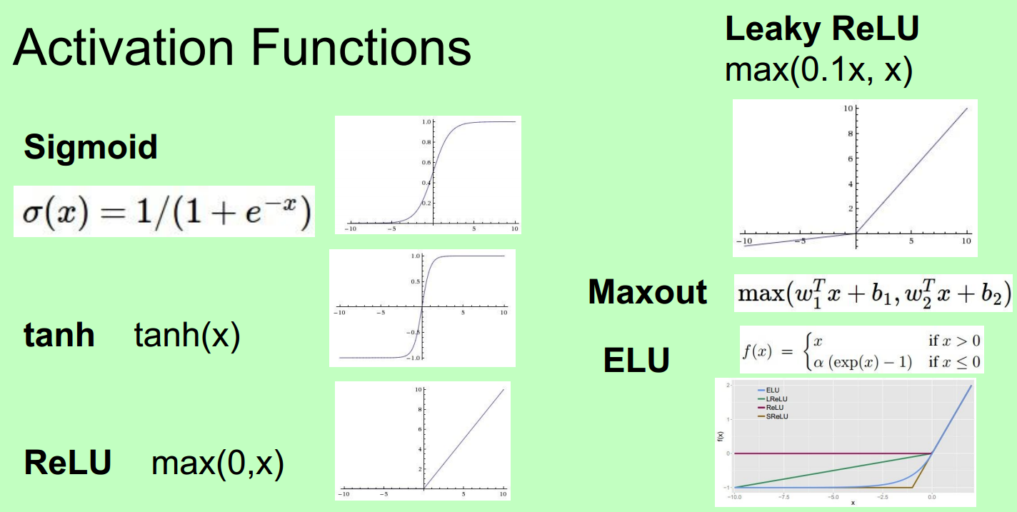
二、讲解
Sigmoid's three problems:
1. Saturated neurons “kill” the gradients
2. Sigmoid outputs are not zerocentered
3. exp() is a bit compute expensive
Tanh 跟sigmoid一样具有毛病1。
Why, “kill” the gradients?

ReLU
Computes f(x) = max(0,x)
- Does not saturate (in +region)
- Very computationally efficient
- Converges much faster than sigmoid/tanh in practice (e.g. 6x)
- Not zero-centered output
- An annoyance: what is the gradient when x < 0? “kill” the gradients. When x = 0, no gradient.
Leaky ReLU
Computes f(x) = max(0.01x, x)
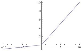
- Does not saturate
- Computationally efficient
- Converges much faster than sigmoid/tanh in practice! (e.g. 6x)
- will not “die”.
Parametric Rectifier (PReLU)
Computes f(x) = max(alpha*x, x)
backprop into \alpha
(parameter)
Exponential Linear Units (ELU)
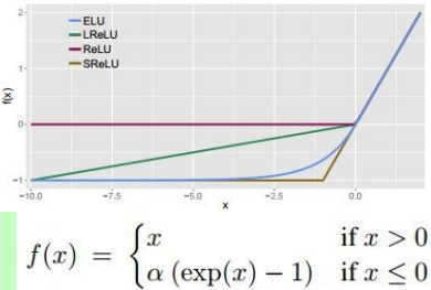
- All benefits of ReLU
- Does not die
- Closer to zero mean outputs
- Computation requires exp()
Maxout “Neuron”
![]()
- Does not have the basic form of dot product ->nonlinearity
- Generalizes ReLU and Leaky ReLU
- Linear Regime! Does not saturate! Does not die!
Problem: doubles the number of parameters/neuron
三、总结:TLDR: In practice
- Use ReLU. Be careful with your learning rates
- Try out Leaky ReLU / Maxout / ELU
- Try out tanh but don’t expect much
- Don’t use sigmoid
预处理

In practice, you may also see PCA and Whitening of the data.
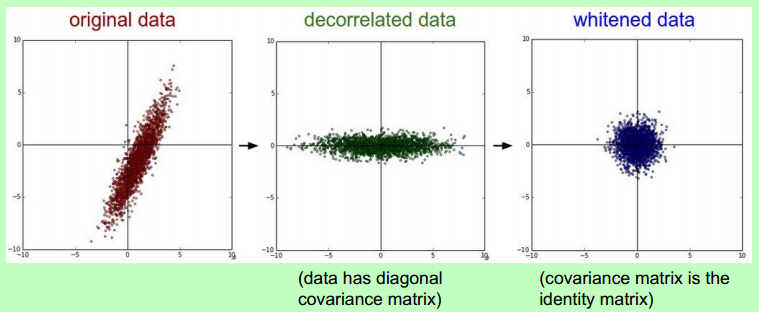
可见,白化的威力!
TLDR: In practice for Images: center only
We don't have separate different features that could be at different units.
Everything is just pixels and they're all bounded between 0 and 255.
So, it is not common to normalize the data, but it's very common to zero center your data.
【以下有点“减小亮度影响”的意思】
- Subtract the mean image (e.g. AlexNet)
(mean image = [32,32,3] array)
- Subtract per-channel mean (e.g. VGGNet)
(mean along each channel = 3 numbers)Not common to normalize variance, to do PCA or whitening.
权重初始化
First idea: Small random numbers
(gaussian with zero mean and 1e-2 standard deviation)
![]()
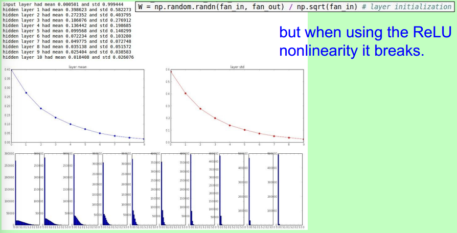
一个十层网络的实验:权重趋于0。

首先,这个实验有必要自己亲自做一下。下图所示,初始值扩大100倍后,几乎所有的neuron趋于饱和,这不利于收敛。

深度网络的调参是个集技术和经验一身的skill,可参见如下的理论。


采用不同的激活函数,得到不同的结果,实践并体会背后的原理。
Proper initialization is an active area of research…
- Understanding the difficulty of training deep feedforward neural networks by Glorot and Bengio, 2010
- Exact solutions to the nonlinear dynamics of learning in deep linear neural networks by Saxe et al, 2013
- Random walk initialization for training very deep feedforward networks by Sussillo and Abbott, 2014
- Delving deep into rectifiers: Surpassing human-level performance on ImageNet classification by He et al., 2015
- Data-dependent Initializations of Convolutional Neural Networks by Krähenbühl et al., 2015
- All you need is a good init, Mishkin and Matas, 2015
Batch Normalization
From: http://blog.csdn.net/hjimce/article/details/50866313
本篇博文主要讲解2015年深度学习领域,非常值得学习的一篇文献:《Batch Normalization: Accelerating Deep Network Training by Reducing Internal Covariate Shift》
附上另一个参考:http://blog.csdn.net/elaine_bao/article/details/50890491 (图示较多)
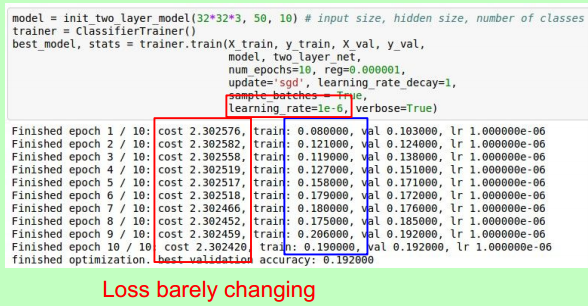
先拿小数据试一试策略,最好能达到overfit (acc = 100%)
以下这个loss不怎么变,可能learning rata太小;
但为什么acc最后突然好了许多?思考。
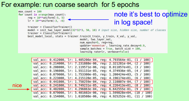
Hyperparameter Optimization
First stage: only a few epochs to get rough idea of what params work
Second stage: longer running time, finer search

参数更新
可见,SGD总是最慢。
注意:加了momentum后的效果;以及改进后的momentum的紫色线(nag)的效果。

唯一的区别在于:
- 传统的:

- 改进的:

然后,通过“变量转换”带来计算上的便利。(nag)

AdaGrad and RMSProp

Adam: 貌似为上策、首选。

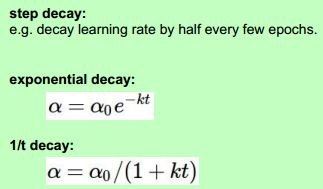
学习率的选择
SGD, SGD+Momentum, Adagrad, RMSProp, Adam all have learning rate as a hyperparameter.
先用快的,再减小,常用策略如下:
Second order optimization methods
- 牛顿法,不需要考虑学习率!
- Quasi-Newton methods (BGFS most popular):
instead of inverting the Hessian (O(n^3)), approximate
inverse Hessian with rank 1 updates over time (O(n^2)
each).
- L-BFGS (Limited memory BFGS):
Does not form/store the full inverse Hessian. Usually works very well in full batch, deterministic mode; not for mini-batch setting.
In practice:
- Adam is a good default choice in most cases
- If you can afford to do full batch updates then try out L-BFGS (and don’t forget to disable all sources of noise)

Regularization (dropout)
Ref: http://www.jianshu.com/p/ba9ca3b07922
总结
- Dropout 方法存在两种形式:直接的和 Inverted。
- 在单个神经元上面,Dropout 方法可以使用伯努利随机变量。
- 在一层神经元上面,Dropout 方法可以使用伯努利随机变量。
- 我们精确的丢弃
np个神经元是不太可能的,但是在一个拥有n个神经元的网络层上面,平均丢弃的神经元就是np个。 - Inverted Dropout 方法可以产生有效学习率。
- Inverted Dropout 方法应该和别的规范化参数的技术一起使用,从而帮助简化学习率的选择过程。
- Dropout 方法有助于防止深度神经网路的过拟合。


