
[Converge] Backpropagation Algorithm
Ref: CS231n Winter 2016: Lecture 4: Backpropagation
Ref: How to implement a NN;中文翻译版本
Ref: Jacobian矩阵和Hessian矩阵
关于这部分内容,请详看链接二内容,并请自在本上手动推导。
理解 Chain Rule

根据Chain Rule进行梯度传递:

 x = 1.37 代入1/x的导数 --> -0.53
 x = 0.37 代入1的导数 乘以 (-0.53) --> -0.53
 x = -1, ex x (-0.53) = e-1 x (-0.53) --> -0.2
 x = 1, 1 * (-1) * (-0.2) --> 0.2
 加号 则可 直接传递下去
 偏导:w0是-1*0.2 = -0.2; x0是2*0.2 = 0.4
-
sigmoid
以下真是一个演示 sigmoid 的伟大例子:

归纳出三个tricky:

代码实现算法
- Part 1: Linear regression
- Intermezzo 1: Logistic classification function
- Part 2: Logistic regression (classification)
- Part 3: Hidden layer
以上部分,总归是对如下代码的理解:
# Python imports
import numpy as np # Matrix and vector computation package
import matplotlib.pyplot as plt # Plotting library
from matplotlib.colors import colorConverter, ListedColormap # some plotting functions
from mpl_toolkits.mplot3d import Axes3D # 3D plots
from matplotlib import cm # Colormaps
# Allow matplotlib to plot inside this notebook
# Set the seed of the numpy random number generator so that the tutorial is reproducable
np.random.seed(seed=1)
# Define and generate the samples
nb_of_samples_per_class = 20 # The number of sample in each class
blue_mean = [0] # The mean of the blue class
red_left_mean = [-2] # The mean of the red class
red_right_mean = [2] # The mean of the red class
std_dev = 0.5 # standard deviation of both classes
# Generate samples from both classes
x_blue = np.random.randn(nb_of_samples_per_class, 1) * std_dev + blue_mean
x_red_left = np.random.randn(nb_of_samples_per_class/2, 1) * std_dev + red_left_mean
x_red_right = np.random.randn(nb_of_samples_per_class/2, 1) * std_dev + red_right_mean
# Merge samples in set of input variables x, and corresponding set of
# output variables t
x = np.vstack((x_blue, x_red_left, x_red_right))
t = np.vstack((np.ones((x_blue.shape[0],1)),
np.zeros((x_red_left.shape[0],1)),
np.zeros((x_red_right.shape[0], 1))))
# 已备齐数据
###############################################################################
# Plot samples from both classes as lines on a 1D space
plt.figure(figsize=(8,0.5))
plt.xlim(-3,3)
plt.ylim(-1,1)
# Plot samples
plt.plot(x_blue, np.zeros_like(x_blue), 'b|', ms = 30)
plt.plot(x_red_left, np.zeros_like(x_red_left), 'r|', ms = 30)
plt.plot(x_red_right, np.zeros_like(x_red_right), 'r|', ms = 30)
plt.gca().axes.get_yaxis().set_visible(False)
plt.title('Input samples from the blue and red class')
plt.xlabel('$x$', fontsize=15)
plt.show()
###############################################################################
# Define the rbf function
def rbf(z):
return np.exp(-z**2)
# Plot the rbf function
z = np.linspace(-6,6,100)
plt.plot(z, rbf(z), 'b-')
plt.xlabel('$z$', fontsize=15)
plt.ylabel('$e^{-z^2}$', fontsize=15)
plt.title('RBF function')
plt.grid()
plt.show()
###############################################################################
# Define the logistic function
def logistic(z):
return 1 / (1 + np.exp(-z))
# Function to compute the hidden activations
def hidden_activations(x, wh):
return rbf(x * wh)
# Define output layer feedforward
def output_activations(h , wo):
return logistic(h * wo - 1)
# Define the neural network function
def nn(x, wh, wo):
return output_activations(hidden_activations(x, wh), wo)
# Define the neural network prediction function that only returns
# 1 or 0 depending on the predicted class
def nn_predict(x, wh, wo):
return np.around(nn(x, wh, wo))
###############################################################################
# Define the cost function
def cost(y, t):
return - np.sum(np.multiply(t, np.log(y)) + np.multiply((1-t), np.log(1-y)))
# Define a function to calculate the cost for a given set of parameters
def cost_for_param(x, wh, wo, t):
return cost(nn(x, wh, wo) , t)
###############################################################################
# Plot the cost in function of the weights
# Define a vector of weights for which we want to plot the cost
nb_of_ws = 200 # compute the cost nb_of_ws times in each dimension
wsh = np.linspace(-10, 10, num=nb_of_ws) # hidden weights
wso = np.linspace(-10, 10, num=nb_of_ws) # output weights
ws_x, ws_y = np.meshgrid(wsh, wso) # generate grid
cost_ws = np.zeros((nb_of_ws, nb_of_ws)) # initialize cost matrix
# Fill the cost matrix for each combination of weights
for i in range(nb_of_ws):
for j in range(nb_of_ws):
cost_ws[i,j] = cost(nn(x, ws_x[i,j], ws_y[i,j]) , t) # 画权值对应的cost等高图,很好的表现方式
# Plot the cost function surface
fig = plt.figure()
ax = Axes3D(fig)
# plot the surface
surf = ax.plot_surface(ws_x, ws_y, cost_ws, linewidth=0, cmap=cm.pink)
ax.view_init(elev=60, azim=-30)
cbar = fig.colorbar(surf)
ax.set_xlabel('$w_h$', fontsize=15)
ax.set_ylabel('$w_o$', fontsize=15)
ax.set_zlabel('$\\xi$', fontsize=15)
cbar.ax.set_ylabel('$\\xi$', fontsize=15)
plt.title('Cost function surface')
plt.grid()
plt.show()
###############################################################################
# Define the error function
def gradient_output(y, t):
return y - t
# Define the gradient function for the weight parameter at the output layer
def gradient_weight_out(h, grad_output):
return h * grad_output
# Define the gradient function for the hidden layer
def gradient_hidden(wo, grad_output):
return wo * grad_output
# Define the gradient function for the weight parameter at the hidden layer
def gradient_weight_hidden(x, zh, h, grad_hidden):
return x * -2 * zh * h * grad_hidden
# Define the update function to update the network parameters over 1 iteration
def backprop_update(x, t, wh, wo, learning_rate):
# Compute the output of the network
# This can be done with y = nn(x, wh, wo), but we need the intermediate
# h and zh for the weight updates.
zh = x * wh
h = rbf(zh) # hidden_activations(x, wh)
y = output_activations(h, wo)
# 以上是正向计算出output的过程
# Compute the gradient at the output
grad_output = gradient_output(y, t) #计算cost
# Get the delta for wo
d_wo = learning_rate * gradient_weight_out(h, grad_output) # <-- 计算w0的改变量
# Compute the gradient at the hidden layer
grad_hidden = gradient_hidden(wo, grad_output)
# Get the delta for wh
d_wh = learning_rate * gradient_weight_hidden(x, zh, h, grad_hidden) # <-- 计算wh的改变量
# return the update parameters
return (wh-d_wh.sum(), wo-d_wo.sum()) # 减小cost,返回更新后的权值对
###############################################################################
# Run backpropagation
# Set the initial weight parameter
wh = 2
wo = -5
# Set the learning rate
learning_rate = 0.2
# Start the gradient descent updates and plot the iterations
nb_of_iterations = 50 # number of gradient descent updates
lr_update = learning_rate / nb_of_iterations # learning rate update rule 设置学习率每次减小的量
w_cost_iter = [(wh, wo, cost_for_param(x, wh, wo, t))] # List to store the weight values over the iterations
for i in range(nb_of_iterations):
learning_rate -= lr_update # decrease the learning rate 学习率在不断的减小
# Update the weights via backpropagation
wh, wo = backprop_update(x, t, wh, wo, learning_rate) # 参数是旧权值,返回了新权值
w_cost_iter.append((wh, wo, cost_for_param(x, wh, wo, t))) # Store the values for plotting
# 通过打印w_cost_iter查看迹线 ----> 见【result】
# Print the final cost
print('final cost is {:.2f} for weights wh: {:.2f} and wo: {:.2f}'.format(cost_for_param(x, wh, wo, t), wh, wo))
###############################################################################
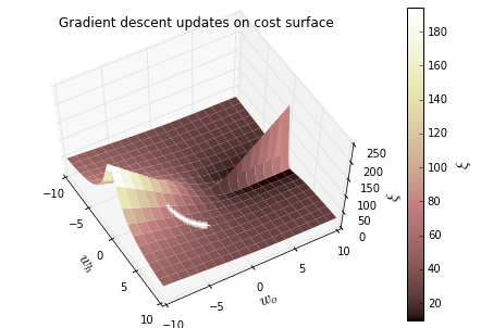
# Plot the weight updates on the error surface
# Plot the error surface
fig = plt.figure()
ax = Axes3D(fig)
surf = ax.plot_surface(ws_x, ws_y, cost_ws, linewidth=0, cmap=cm.pink)
ax.view_init(elev=60, azim=-30)
cbar = fig.colorbar(surf)
cbar.ax.set_ylabel('$\\xi$', fontsize=15)
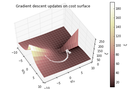
# Plot the updates
for i in range(1, len(w_cost_iter)):
wh1, wo1, c1 = w_cost_iter[i-1]
wh2, wo2, c2 = w_cost_iter[i]
# Plot the weight-cost value and the line that represents the update
ax.plot([wh1], [wo1], [c1], 'w+') # Plot the weight cost value
ax.plot([wh1, wh2], [wo1, wo2], [c1, c2], 'w-')
# Plot the last weights
wh1, wo1, c1 = w_cost_iter[len(w_cost_iter)-1]
ax.plot([wh1], [wo1], c1, 'w+')
# Shoz figure
ax.set_xlabel('$w_h$', fontsize=15)
ax.set_ylabel('$w_o$', fontsize=15)
ax.set_zlabel('$\\xi$', fontsize=15)
plt.title('Gradient descent updates on cost surface')
plt.grid()
plt.show()
Result: 学习率不同

再添加一层隐藏层,如下,推导后可见递推过程:

“多分类” Softmax代码实现
# Python imports
import numpy as np # Matrix and vector computation package
import matplotlib.pyplot as plt # Plotting library
from matplotlib.colors import colorConverter, ListedColormap # some plotting functions
from mpl_toolkits.mplot3d import Axes3D # 3D plots
from matplotlib import cm # Colormaps
# Allow matplotlib to plot inside this notebook
###############################################################################
# Define the softmax function
def softmax(z):
return np.exp(z) / np.sum(np.exp(z))
###############################################################################
# Plot the softmax output for 2 dimensions for both classes
# Plot the output in function of the weights
# Define a vector of weights for which we want to plot the ooutput
nb_of_zs = 200
zs = np.linspace(-10, 10, num=nb_of_zs) # input
zs_1, zs_2 = np.meshgrid(zs, zs) # generate grid
# 200*200的矩阵
y = np.zeros((nb_of_zs, nb_of_zs, 2)) # initialize output
# Fill the output matrix for each combination of input z's
for i in range(nb_of_zs):
for j in range(nb_of_zs):
y[i,j,:] = softmax( np.asarray( [zs_1[i,j], zs_2[i,j]] ) )
# Grid上的某个像素点的坐标值天然地代表两个值
# 将两值通过softmax转换后获得对比结果
###############################################################################
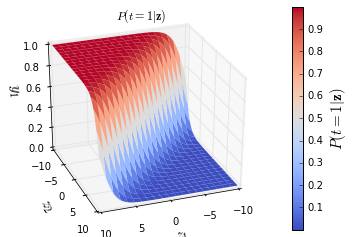
# Plot the cost function surfaces for both classes
fig = plt.figure()
# Plot the cost function surface for t=1
ax = fig.gca(projection='3d')
surf = ax.plot_surface(zs_1, zs_2, y[:,:,0], linewidth=0, cmap=cm.coolwarm)
ax.view_init(elev=30, azim=70)
cbar = fig.colorbar(surf)
ax.set_xlabel('$z_1$', fontsize=15)
ax.set_ylabel('$z_2$', fontsize=15)
ax.set_zlabel('$y_1$', fontsize=15)
ax.set_title ('$P(t=1|\mathbf{z})$')
cbar.ax.set_ylabel('$P(t=1|\mathbf{z})$', fontsize=15)
plt.grid()
plt.show()
###############################################################################
Result:
注解:


zs_1
Out[49]:
array([[-10.        ,  -9.89949749,  -9.79899497, ...,   9.79899497,
          9.89949749,  10.        ],
       [-10.        ,  -9.89949749,  -9.79899497, ...,   9.79899497,
          9.89949749,  10.        ],
       [-10.        ,  -9.89949749,  -9.79899497, ...,   9.79899497,
          9.89949749,  10.        ],
       ...,
       [-10.        ,  -9.89949749,  -9.79899497, ...,   9.79899497,
          9.89949749,  10.        ],
       [-10.        ,  -9.89949749,  -9.79899497, ...,   9.79899497,
          9.89949749,  10.        ],
       [-10.        ,  -9.89949749,  -9.79899497, ...,   9.79899497,
          9.89949749,  10.        ]])

zs_2
Out[50]:
array([[-10.        , -10.        , -10.        , ..., -10.        ,
        -10.        , -10.        ],
       [ -9.89949749,  -9.89949749,  -9.89949749, ...,  -9.89949749,
         -9.89949749,  -9.89949749],
       [ -9.79899497,  -9.79899497,  -9.79899497, ...,  -9.79899497,
         -9.79899497,  -9.79899497],
       ...,
       [  9.79899497,   9.79899497,   9.79899497, ...,   9.79899497,
          9.79899497,   9.79899497],
       [  9.89949749,   9.89949749,   9.89949749, ...,   9.89949749,
          9.89949749,   9.89949749],
       [ 10.        ,  10.        ,  10.        , ...,  10.        ,
         10.        ,  10.        ]])
关于softmax激活函数对于自变量z的求导过程如下:

采用矢量化的表示
一、正向传播

01. node.
我们有N个输入数据,每个数据有两个可能的类别选项,那么我们可以得到矩阵X(输入数据)如下:

其中,xij表示第i个样本的第j个类别选项的概率。
经过softmax函数之后,该模型输出的最终结果T为:

其中,当且仅当第i个样本属于类别j时,tij=1。
因此,我们定义
- 蓝色样本的标记是
T = [0 1], - 红色样本的标记是
T = [1 0]
02. edge.

03. node and edge --> values on hidden layer


04. output layer

之后计算结果如下:

助解:
- 不同行代表不同样本。
- 每一行给出两个概率值。
二、反向传播
-
如何计算误差
如果需要对N个样本进行C个分类,那么它的损失函数ξ是:【cross-entropy】

损失函数的误差梯度δo可以非常方便得到:

具体推导过程如下


其中,Zo(Zo=H⋅Wo+bo)是一个n*2的矩阵,
[Y:是一个经过模型得到的n*2的输出矩阵] - [T:是一个n*2的目标矩阵]
因此,δo 也是一个n*2的矩阵。
-
如何更新权重(仅输出层)
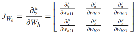
对于N个样本,对输出层的梯度δwoj是通过∂ξ/∂woj计算的,具体计算如下:

其中,woj表示Wo的第j行,即是一个1*2的向量。因此,我们可以将上式改写成一个矩阵操作,即:

最后梯度的结果是一个3*2的Jacobian矩阵,如下:

-
如何更新偏差项(仅输出层)
对于偏差项bo可以采用相同的方式进行更新。对于批处理的N个样本,对输出层的梯度∂ξ/∂bo的计算如下:

最后梯度的结果是一个2*1的Jacobian矩阵,如下:

-
如何更新权重(Hidden Layer)
-
如何更新偏差项(Hidden Layer)

三、梯度检查
在编程计算反向传播梯度时,很容易产生错误。这就是为什么一直推荐在你的模型中一定要进行梯度检查。
梯度检查是通过对于每一个参数进行梯度数值计算进行的,即检查这个数值与通过反向传播的梯度进行比较计算。
对于每个参数的数值梯度应该接近于反向传播梯度的参数。
Ref: http://blog.csdn.net/u012526120/article/details/48973497
对于一个函数来说,通常有两种计算梯度的方式:
-
- 数值梯度(numerical gradient);
- 解析梯度(analytic gradient);
From 231n Lec03

###############################################################################
# Gradient checking
###############################################################################

# Combine all parameter matrices in a list
# Combine all parameter gradients in a list
params      = [Wh, bh, Wo, bo]
grad_params = [JWh, Jbh, JWo, Jbo]


# Set the small change to compute the numerical gradient
eps = 0.0001

# Check each parameter matrix
for p_idx in range(len(params)):
    # Check each parameter in each parameter matrix
    for row in range(params[p_idx].shape[0]):
        for col in range(params[p_idx].shape[1]):
            # 遍历(检查)每一个矩阵的每一个元素

            # Copy the parameter matrix and change the current parameter slightly
            p_matrix_min = params[p_idx].copy()
            p_matrix_min[row,col] -= eps
            p_matrix_plus = params[p_idx].copy()
            p_matrix_plus[row,col] += eps

            # Copy the parameter list, and change the updated parameter matrix
            params_min = params[:]
            params_min[p_idx]  = p_matrix_min
            params_plus = params[:]
            params_plus[p_idx] =  p_matrix_plus


            # Compute the numerical gradient 计算数值梯度
            grad_num = ( cost(nn(X, *params_plus), T) - cost(nn(X, *params_min), T) )/(2*eps)

            # cost(交叉entropy误差); nn(计算正向传播输出)

            # Raise error if the numerical grade is not close to the backprop gradient
            if not np.isclose(grad_num, grad_params[p_idx][row,col]):
                raise ValueError('Numerical gradient of {:.6f} is not close to the backpropagation gradient of {:.6f}!'.format(float(grad_num), float(grad_params[p_idx][row,col])))
print('No gradient errors found')
计算数值梯度
![]()
grad_num, grad_params[p_idx][row,col]对比如下,可见十分接近。
0.0469372659495
0.0469372661302

0.808593180182
0.808593180814

-0.0596231433292
-0.0596231429511

-0.091797324302
-0.0917973244116

-0.348418390672
-0.348418391494

0.523644930297
0.523644931161

1.57820501329
1.57820501394

-8.92123130654
-8.92123130677

15.5379406418
15.5379406533

-19.8494527815
-19.8494527829

19.8494527815
19.8494527829

-23.0447452795
-23.0447452822

23.0447452795
23.0447452822

-23.6601089617
-23.6601089633

23.6601089617
23.6601089633

-43.2009781318
-43.2009781406

43.2009781319
43.2009781406
四、动量方法
定义速度:(初始化)
Wh
array([[-9.02740895,  0.98074176, -8.04226996],
       [-4.07352687,  9.53464723,  5.84734039]])

bh
array([[-4.63991557, -5.38003474,  4.98589781]])

Wo
array([[ 8.05340601, -7.95188719],
       [ 8.18246481, -8.23254238],
       [-8.08833273,  8.01526731]])

bo
array([[ 3.41333769, -3.31267928]])

#############################################################################
Vs = [np.zeros_like(M) for M in [Wh, bh, Wo, bo]]

Vs
[array([[ 0.,  0.,  0.], [ 0.,  0.,  0.]]),
 array([[ 0.,  0.,  0.]]),
 array([[ 0.,  0.], [ 0.,  0.], [ 0.,  0.]]),
 array([[ 0.,  0.]])]
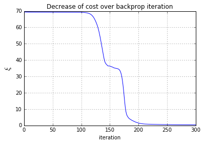
# Start the gradient descent updates and plot the iterations
nb_of_iterations = 300  # number of gradient descent updates
ls_costs = [cost(nn(X, Wh, bh, Wo, bo), T)]  # list of cost over the iterations

for i in range(nb_of_iterations):
    # Update the velocities and the parameters

    Vs = update_velocity(X, T, [Wh, bh, Wo, bo], Vs, momentum_term, learning_rate)  # 先得到 new v
    Wh, bh, Wo, bo = update_params([Wh, bh, Wo, bo], Vs)                            # 加入new v,求new param

    ls_costs.append(cost(nn(X, Wh, bh, Wo, bo), T))
核心函数分析:
# Define the update function to update the network parameters over 1 iteration
# 一次迭代后获得的各层梯度,也就是Jacabian matrix
def backprop_gradients(X, T, Wh, bh, Wo, bo):
    # Compute the output of the network
    # Compute the activations of the layers
    H = hidden_activations(X, Wh, bh)
    Y = output_activations(H, Wo, bo)

    # Compute the gradients of the output layer
    Eo  = error_output(Y, T)
    JWo = gradient_weight_out(H, Eo)
    Jbo = gradient_bias_out(Eo)

    # Compute the gradients of the hidden layer
    Eh  = error_hidden(H, Wo, Eo)
    JWh = gradient_weight_hidden(X, Eh)
    Jbh = gradient_bias_hidden(Eh)

    return [JWh, Jbh, JWo, Jbo]  # Jeff:每层俩参数,两层就是四个

def update_velocity(X, T, ls_of_params, Vs, momentum_term, learning_rate):
    # ls_of_params = [Wh, bh, Wo, bo]
    # Js = [JWh, Jbh, JWo, Jbo]
    Js = backprop_gradients(X, T, *ls_of_params)

return [momentum_term * V - learning_rate * J for V,J in zip(Vs, Js)]

def update_params(ls_of_params, Vs):
    # ls_of_params = [Wh, bh, Wo, bo]
    # Vs = [VWh, Vbh, VWo, Vbo]

return [P + V for P,V in zip(ls_of_params, Vs)]
加了惯性后的梯度下降迹线图:(是有点不同的感觉)
五、参数的可视化
-
可视化训练分类结果
# Plot the resulting decision boundary
# Generate a grid over the input space to plot the color of the
#  classification at that grid point
nb_of_xs = 200
xs1 = np.linspace(-2, 2, num=nb_of_xs)
xs2 = np.linspace(-2, 2, num=nb_of_xs)
xx, yy = np.meshgrid(xs1, xs2) # create the grid

# Initialize and fill the classification plane
classification_plane = np.zeros((nb_of_xs, nb_of_xs))
for i in range(nb_of_xs):
    for j in range(nb_of_xs):
        pred = nn_predict(np.asmatrix([xx[i,j], yy[i,j]]), Wh, bh, Wo, bo)
        classification_plane[i,j] = pred[0,0]  #这里只需要判断一个elem就好了

# classification_plane构成的密集网格点,计算每个点的分类结果

# Create a color map to show the classification colors of each grid point
cmap = ListedColormap([
        colorConverter.to_rgba('b', alpha=0.30),
        colorConverter.to_rgba('r', alpha=0.30)])

# Plot the classification plane with decision boundary and input samples
plt.contourf(xx, yy, classification_plane, cmap=cmap)
# 对二值图找轮廓 <---

# Plot both classes on the x1, x2 plane
plt.plot(x_red[:,0], x_red[:,1], 'ro', label='class red')
plt.plot(x_blue[:,0], x_blue[:,1], 'bo', label='class blue')
plt.grid()
plt.legend(loc=1)
plt.xlabel('$x_1$', fontsize=15)
plt.ylabel('$x_2$', fontsize=15)
plt.axis([-1.5, 1.5, -1.5, 1.5])
plt.title('red vs blue classification boundary')
plt.show()
NB: nn_predict时,需要改变为 keepdims=False,如下:
# Define the softmax function
def softmax(z):
    return np.exp(z) / np.sum(np.exp(z), axis=1, keepdims=True))
pred = nn_predict(np.asmatrix([xx[1,1], yy[1,1]]), Wh, bh, Wo, bo)

pred
Out[162]: matrix([[ 1.,  0.]])

pred[0,0]  # 这里只需看一个就好,另一个肯定是相反的
Out[163]: 1.0
-
输入域的转换(隐藏层的升维效果)
# Plot the projection of the input onto the hidden layer

# Define the projections of the blue and red classes
H_blue = hidden_activations(x_blue, Wh, bh)
H_red  = hidden_activations(x_red, Wh, bh)
#

# Plot the error surface
fig = plt.figure()
ax  = Axes3D(fig)
ax.plot(np.ravel(H_blue[:,0]), np.ravel(H_blue[:,1]), np.ravel(H_blue[:,2]), 'bo')
ax.plot(np.ravel(H_red[:,0]),  np.ravel(H_red[:,1]),  np.ravel(H_red[:,2]),  'ro')

ax.set_xlabel('$h_1$', fontsize=15)
ax.set_ylabel('$h_2$', fontsize=15)
ax.set_zlabel('$h_3$', fontsize=15)

ax.view_init(elev=10, azim=-40)
plt.title('Projection of the input X onto the hidden layer H')
plt.grid()
plt.show()
思考,这样的数据表现对理解有什么帮助?
-- 升维后,貌似成为了超平面可分!

参见:http://cs.stanford.edu/people/karpathy/convnetjs/demo/classify2d.html
思考题
"不管层数增加几层,只要不升维,就是不能分类,为什么?“
六、更多层的网络
My node:
-
- 第一,在一个大型的训练数据集上面,我们可以节省时间和内存,因为这个算法减少了很多的矩阵操作。
- 第二,增加了训练样本的多样性。
后记:
本文只是一个非常非常简要的阅读笔记。Peter Roelants的这系列博文需要认认真真在本子上推导,并总结相关细节操作。
这些操作在tensorflow上可能只是某个参数的设置,但原理的深刻理解决定了在该领域的发展上限。

 浙公网安备 33010602011771号