
Stanford coursera Andrew Ng 机器学习课程编程作业(Exercise 1)
Exercise 1:Linear Regression---实现一个线性回归
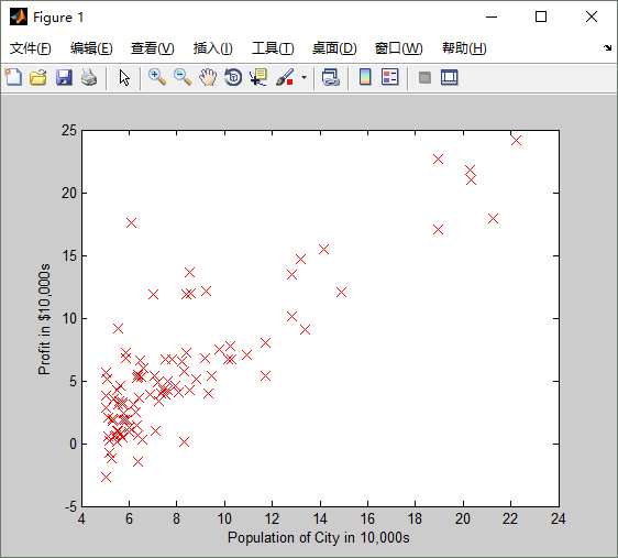
在本次练习中,需要实现一个单变量的线性回归。假设有一组历史数据<城市人口,开店利润>,现需要预测在哪个城市中开店利润比较好?
历史数据如下:第一列表示城市人口数,单位为万人;第二列表示利润,单位为10,000$
    5.5277    9.1302
    8.5186   13.6620
    7.0032   11.8540
    .....
    ......
用Matlab画出的图形如下:首先加载数据,将data中的第一列数据保存到X中,将data中的所有行的第2列数据保存到y中
data = load('ex1data1.txt'); %加载数据
X = data(:, 1); y = data(:, 2);
m = length(y); % number of training examples

% Plot Data
% Note: You have to complete the code in plotData.m
plotData(X, y);
plotData.m代码如下:执行plot函数画图;xlabel、ylabel分别给X轴和Y轴标记提示信息。
function plotData(x, y)
%PLOTDATA Plots the data points x and y into a new figure
%   PLOTDATA(x,y) plots the data points and gives the figure axes labels of
%   population and profit.

% ====================== YOUR CODE HERE ======================
% Instructions: Plot the training data into a figure using the
%               "figure" and "plot" commands. Set the axes labels using
%               the "xlabel" and "ylabel" commands. Assume the
%               population and revenue data have been passed in
%               as the x and y arguments of this function.
%
% Hint: You can use the 'rx' option with plot to have the markers
%       appear as red crosses. Furthermore, you can make the
%       markers larger by using plot(..., 'rx', 'MarkerSize', 10);

figure; % open a new figure window

plot(x,y,'rx','MarkerSize',10);
ylabel('Profit in $10,000s');
xlabel('Population of City in 10,000s');

% ============================================================

end
画出来的图形如下:
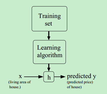
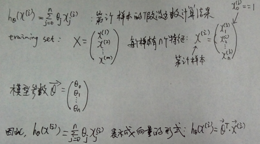
①假设函数(hypothesis function)
在给定一些样本数据(training set)后,采用某种学习算法(learning algorithm)对样本数据进行训练,得到了一个模型或者说是假设函数。
当需要预测新数据的结果时,将新数据作为假设函数的输入,假设函数计算后得到结果,这个结果就作为预测值。
假设函数的表示形式一般如下:θ 称为模型的参数(或者是:权重weights),x就是输入变量(input variables or feature variables)
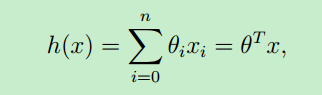
可以看出,假设函数h(x)是关于x的函数,只要确定了 θ ,就求得了假设函数 (θ 也可视为一个向量)。那么对于新的输入样本x,就可以预测该样本的结果y了。
上面假设函数是从0到n求和,也就是说:对于每个输入样本x,将它看成一个向量,每个x中有n+1个 features。比如预测房价,那输入的样本 x(房子的大小,房子所在的城市,卫生间个数,阳台个数.....一系列的特征)
关于分类问题和回归问题:假设函数的输出结果y(predicted y)有两种表示形式:离散的值和连续的值。比如本文中讲到的预测利润,这个结果就是属于连续的值;再比如说根据历史的天气情况预测明天的天气(下雨 or 不下雨),那预测的结果就是离散的值(discrete values)
因此,若hypothesis function输出是连续的值,则称这类学习问题为回归问题(regression problem),若输出是离散的值,则称为分类问题(classification problem)
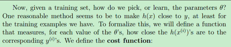
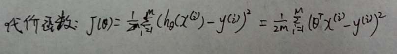
②代价函数(cost function)
学习过程就是确定假设函数的过程,或者说是:求出 θ 的过程。
现在先假设 θ 已经求出来了,就需要判断求得的这个假设函数到底好不好?它与实际值的偏差是多少?因此,就用代价函数来评估。
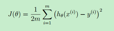
一般地,用 m 来表示训练样本的数目(size of training set),x(i) 表示第 i 个样本,y(i) 表示第i个样本的预测结果。
从上图可看出:代价函数与“最小均方差”的理念非常相似。J(θ)是 θ 函数。
显然,“代价函数越小,模型就越好”。因此,目标就是:找到一组合适的 θ ,使得代价函数取最小值。
如果我们找到了 θ ,那不就求得了 假设函数了?也就求得一个模型--linear regression model.
那如何找 θ 呢?就是下面提到的梯度下降算法(Gradient descent algorithm)
③梯度下降算法(Gradient descent algorithm)
梯度下降算法的本质就是求偏导数,令偏导数等于0,解出 θ
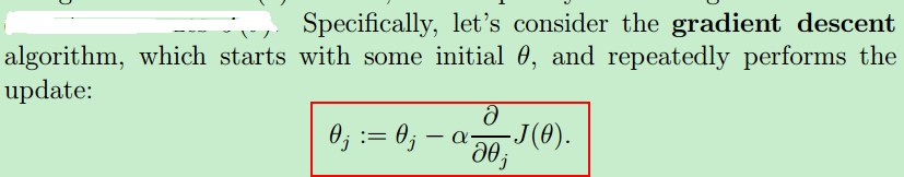
首先从一个初始 θ 开始,然后 for 循环执行上面公式,当偏导数等于0时,θj 就不会再更新了,此时就得到一个最终θj 值。
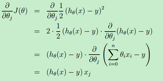
整个偏导数的运算过程如下:
④假设函数、代价函数和梯度下降算法的向量表示
假设函数的向量表示如下:
代价函数的表示如下:
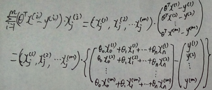
使用梯度下降算法求解 θ 的向量表示如下:
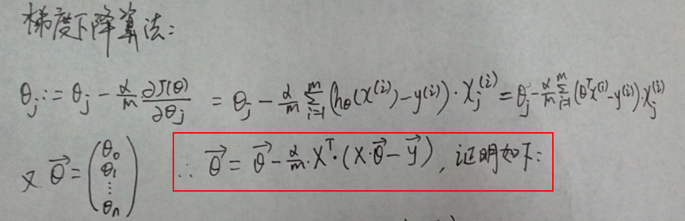
证明过程如下:

⑤Matlab语言表示 代价函数和梯度下降算法
梯度下降算法表示如下:(gradientDescent.m)
function [theta, J_history] = gradientDescent(X, y, theta, alpha, num_iters)
%GRADIENTDESCENT Performs gradient descent to learn theta
%   theta = GRADIENTDESENT(X, y, theta, alpha, num_iters) updates theta by
%   taking num_iters gradient steps with learning rate alpha

% Initialize some useful values
m = length(y); % number of training examples
J_history = zeros(num_iters, 1);

for iter = 1:num_iters
    theta = theta - (alpha/m)*X'*(X*theta-y); % theta 就是用上面的向量表示法的 matlab 语言实现
    % ====================== YOUR CODE HERE ======================
    % Instructions: Perform a single gradient step on the parameter vector
    %               theta.
    %
    % Hint: While debugging, it can be useful to print out the values
    %       of the cost function (computeCost) and gradient here.
    %
    % ============================================================

    % Save the cost J in every iteration
    J_history(iter) = computeCost(X, y, theta);

end

end
代价函数表示如下:(computeCost.m)
function J = computeCost(X, y, theta)
%COMPUTECOST Compute cost for linear regression
%   J = COMPUTECOST(X, y, theta) computes the cost of using theta as the
%   parameter for linear regression to fit the data points in X and y

% Initialize some useful values
m = length(y); % number of training examples

% You need to return the following variables correctly
J = 0;

% ====================== YOUR CODE HERE ======================
% Instructions: Compute the cost of a particular choice of theta
%               You should set J to the cost.
J = sum((X*theta-y).^2)/(2*m);
% =========================================================================

end
运行上面的Matlab程序,求得的线性回归模型如下图:

它的一个预测结果如下:
For population = 35,000, we predict a profit of 4519.767868
For population = 70,000, we predict a profit of 45342.450129
代价函数J(θ0 , θ1)的图形如下:(因为我们只有一个特征变量(population)--不考虑x0)。因此,共有两个模型参数,θ0对应着x0, θ1对应着x1

两个变量:θ0 , θ1,因此画出来的图形可用三维空间来表示。
原文:http://www.cnblogs.com/hapjin/p/6079012.html

 浙公网安备 33010602011771号