学习笔记 | Udacity CarND Term3: Path Planning, Concentration and Systems

Udacity CarND Term3: Path Planning, Concentration and Systems

Overview (1/4/2018 - 4/10/2018)

Welcome (1/4/2018)
Search (1/4/2018 - 1/7/2018)
Prediction (1/14/2018 - 1/15/2018; 1/16/2018) implementation of gnb clssifier
Behavior Planning (1/14/2018 - 1/15/2018; 1/17/2018) L10: Behavior Planning Psudocode; L13-16: Cost function; L20-21: Behavior Planner
Trajectory Generation (1/14/2018 - 1/15/2018) L13-14, 26-27, 32
Project: Path Planning Project (1/17/2018 - )
Coming up: Electives (1/6/2018)
Elective: Advanced Deep Learning (1/6/2018)
Fully Convolutional Networks (1/6/2018)
Scene Understanding (1/6/2018)
Inference Performance (1/7/2018)
Project: Semantic Segmantation Project (1/13/2018 - 1/16/2018)
Elective: Functional Safety
Introduction to Functional Safety
Functional Safety: Safety Plan
Functional Safety: Hazard Analysis and Risk Assessment
Functional Safety: Functional Safety Concept
Functional Safety: Techinical Safety Concept
Functional Safety at the Sofware and Hardware Levels
Project: Elective Project: Functional Safety
Autonomous Vehicle Architecture (1/5/2018)
Introduction to ROS (1/5/2018)
Packages and Catkin Workspaces (1/5/2018)
Writting ROS Nodes (1/15/2018)
Project: System Integration Project
Complete the Program

Note

2. Search

A* Algorithm
Dynamic Programming

3. Prediction

Frenet Coordinates ---- a very convenient method to represent car's longitude displacement and lateral displacement
Multimodel Estimation
Data-Driven Approaches
- Data-driven approaches solve the prediction problem in two phases:
  1. Offline training
  2. Online Prediction
- Offline Training
  - In this phase the goal is to feed some machine learning algorithm a lot of data to train it. For the trajectory clustering example this involved:
    1. Define similarity - we first need a definition of similarity that agrees with human common-sense definition.
    2. Unsupervised clustering - at this step some machine learning algorithm clusters the trajectories we've observed.
    3. Define Prototype Trajectories - for each cluster identify some small number of typical "prototype" trajectories.
- Online Prediction
  - Once the algorithm is trained we bring it onto the road. When we encounter a situation for which the trained algorithm is appropriate (returning to an intersection for example) we can use that algorithm to actually predict the trajectory of the vehicle. For the intersection example this meant:
    1. Observe Partial Trajectory - As the target vehicle drives we can think of it leaving a "partial trajectory" behind it.
    2. Compare to Prototype Trajectories - We can compare this partial trajectory to the corresponding parts of the prototype trajectories. When these partial trajectories are more similar (using the same notion of similarity defined earlier) their likelihoods should increase relative to the other trajectories.
    3. Generate Predictions - For each cluster we identify the most likely prototype trajectory. We broadcast each of these trajectories along with the associated probability (see the image below).

Model Based Approaches
- You can think of model based solutions to the prediction problem as also having an "offline" and online component. In that view, this approach requires:
  1. Defining process models (offline).
  2. Using process models to compare driver behavior to what would be expected for each model.
  3. Probabilistically classifying driver intent by comparing the likelihoods of various behaviors with a multiple-model algorithm.
  4. Extrapolating process models to generate trajectories.

4. Behavior Planning

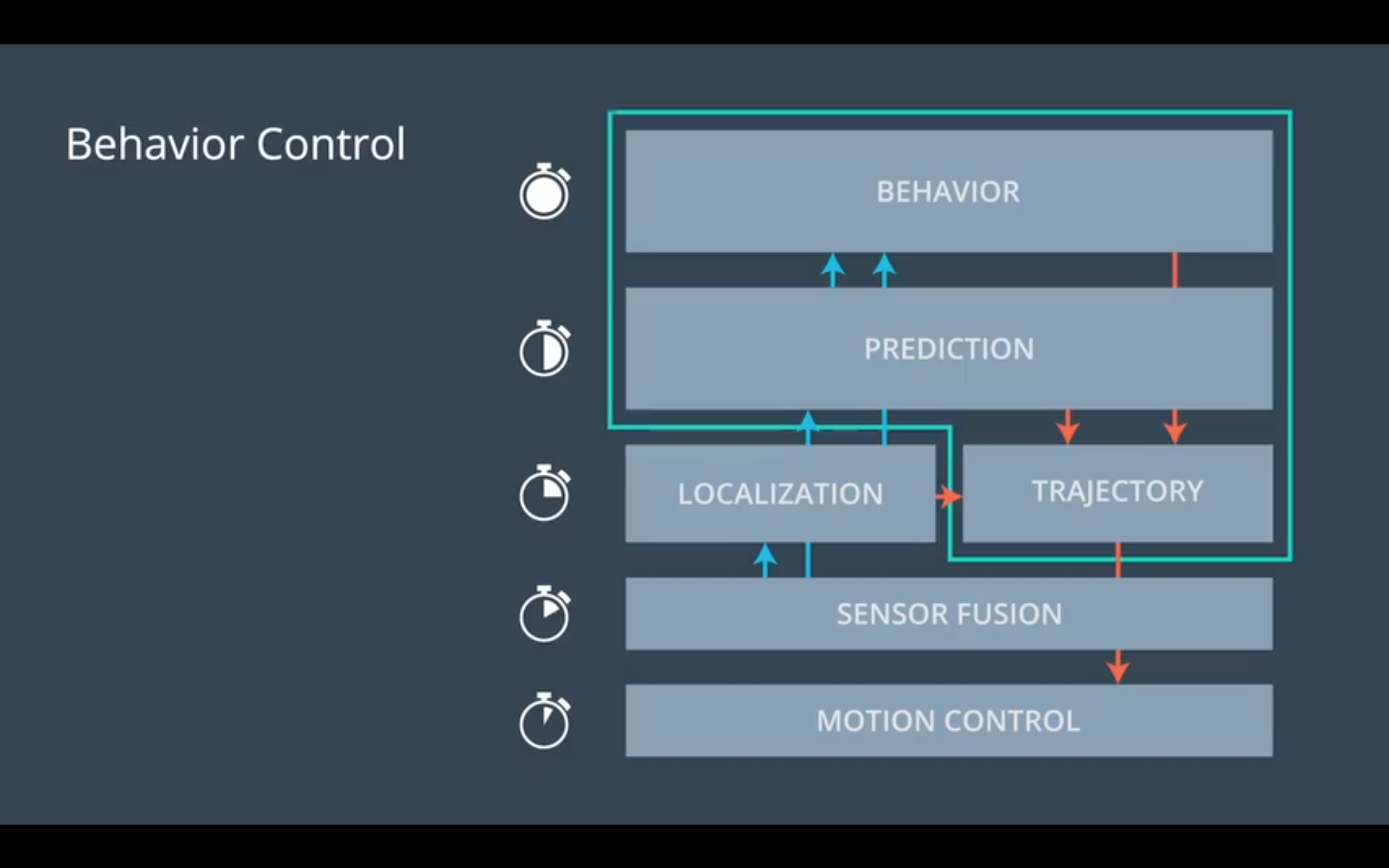
Behavior Control
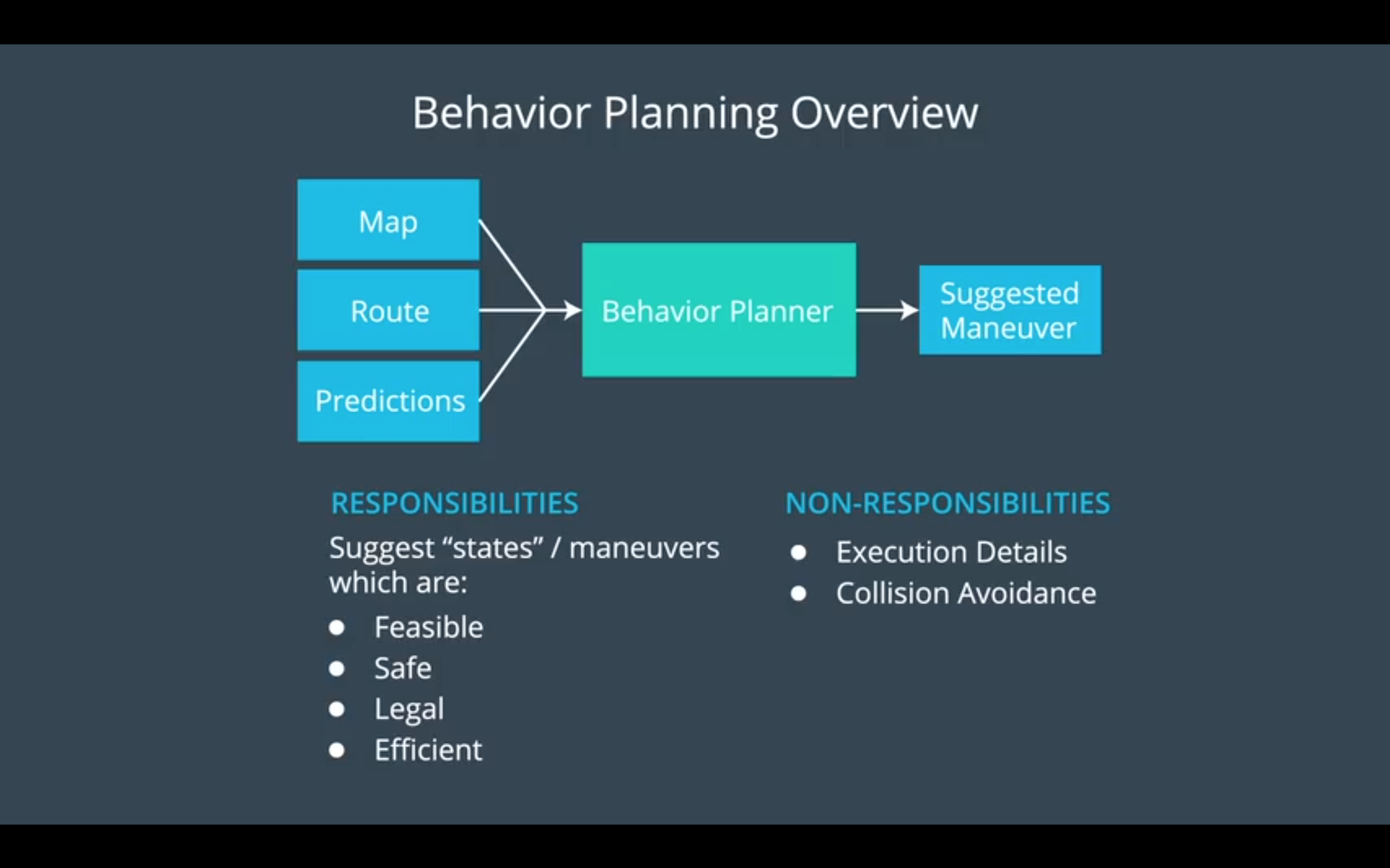
Behavior Planing Overview

5. Trajectory Generation

6. Project: Path Planning Project

centripetal acceleration 向心加速度
jerk 颠簸地行进
Walkthrough video
- [00:00 - 02:45] Introduce the starter code.
- [02:46 - 05:54] main.cpp -> helper functions
- [05:55 - 08:00] main.cpp -> main function: load map data, get car's location (in "telemetry" block), sensor fusion block
- [08:00 - 11:22] main function: next_x, next_y. Create a straight trajectory to simply make it move.
  - ```
  double dist_inc = 0.5;
  for(int i = 0; i < 50; i++)
  {
       next_x_vals.push_back(car_x+(dist_inc*i)*cos(deg2rad(car_yaw)));
       next_y_vals.push_back(car_y+(dist_inc*i)*sin(deg2rad(car_yaw)));
  }
```
- [11:23 - 17:40] main function: next_x, next_y. Update the trajectory to lane keep with frenet transformation.
  - ```
  double dist_inc = 0.5;
  for(int i = 0; i < 50; i++)
  {
      double next_s = car_s + (i + 1) * dist_inc;
      double next_d = 6;
      vector<double> xy = getXY(next_s, next_d, map_waypoints_s, map_waypoints_x, map_waypoints_y);
  
      next_x_vals.push_back(xy[0]);
      next_y_vals.push_back(xy[1]);
  }
```
- [17:41 - 18:55] driving slowly
- [18:56 - 39:50] smooth the path or minimize the jerk (lesson ?), spline library, polynomial fits. We use spline instead of polynomial since it is easy to use the library.
- [39:51 - 48:44] checking cars in front and slow down to avoid hitting the other cars
- [48:45 - 52:50] solving the "cold start" problem by defining very small accelaration
- [52:51 - 57:00] a basic lane change
- [57:01 - 58:40] general idea of incorparating behavior planner
- [58:40 - end] questions

9. Fully Convolutional Networks

"fully-connected layers" --> "1-by-1 convolutions"

from a fully-connected layer to a 1-by-1 convolution in TensorFlow:

num_classes = 2
output = tf.layers.dense(input, num_classes)

To:

num_classes = 2
output = tf.layers.conv2d(input, num_classes, 1, strides=(1,1))

3 points in FCN
1. one by one (1x1) convolutional layers (replacing fully connected layers)
2. up-sampling through the use of transposed convolutional layers (or de-concolutional layers)
3. skip connection (here to restore the spatial information)
How one by one convolution works? Check this: One by One [ 1 x 1 ] Convolution - counter-intuitively useful
The architecture of FCN
- Encoder ---> Decoder (shown as the below picture)
- The encoder is Convolutional network which is to extract features from the image and can use Transfer Learning. VGG and ResNet are often used.
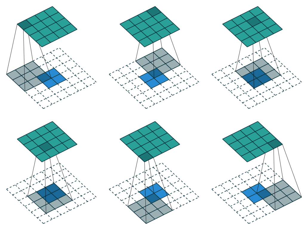
- The decoder is a Decovolutional network which is also called transposed convolution
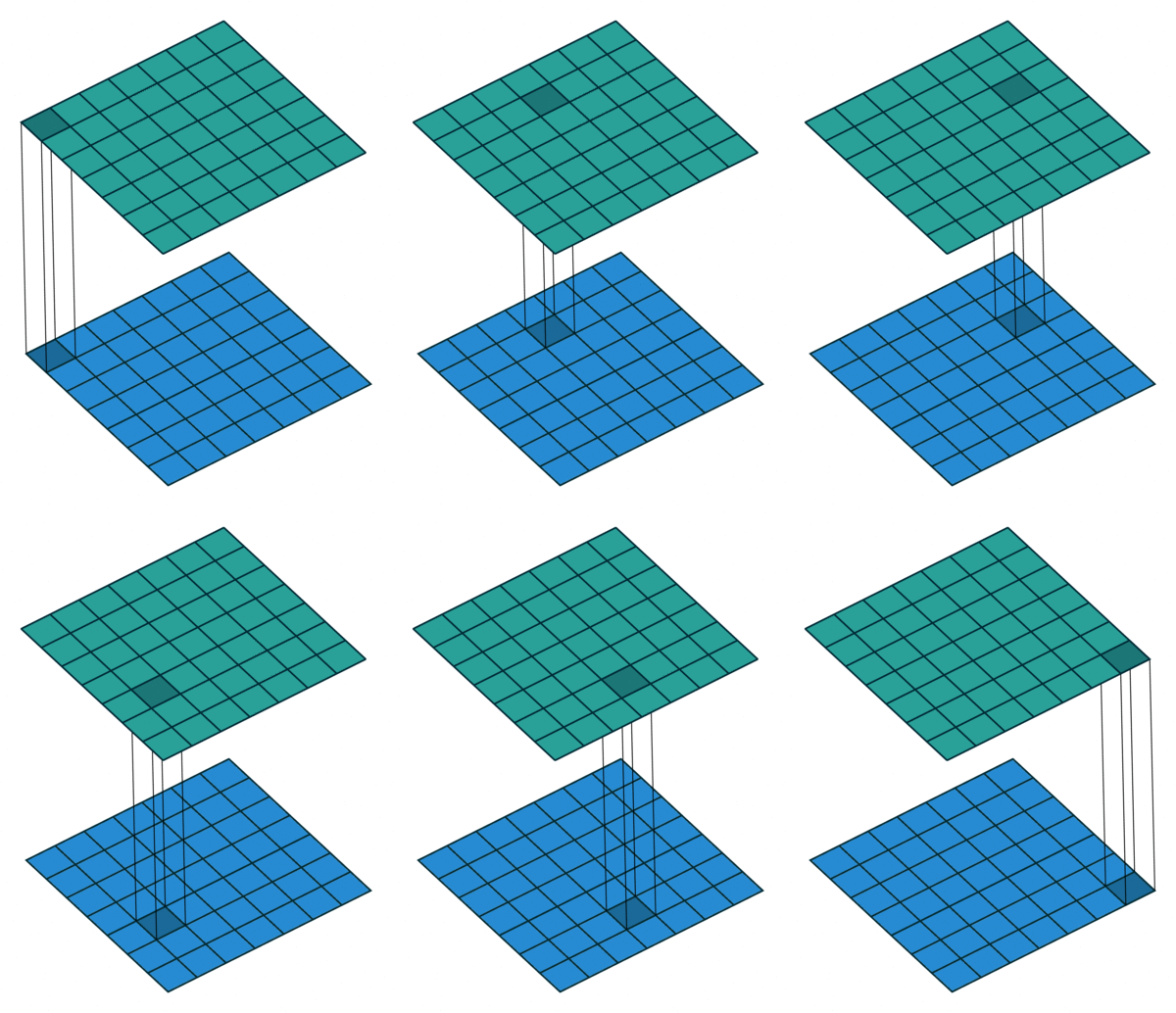
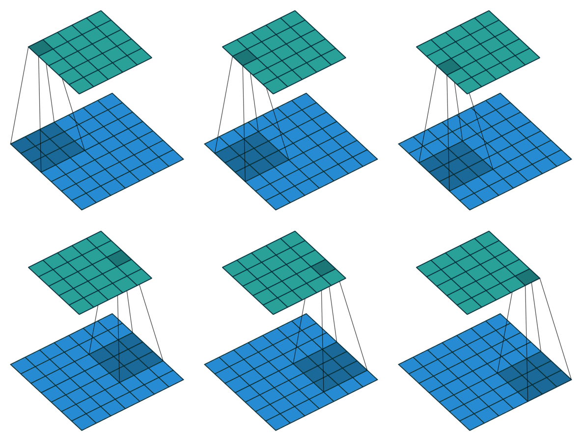
- Convolution & Deconvolution Display

- tf.layers.conv2d(x, num_outputs, 1, 1, weights_initializer=custom_init)
  - num_outputs defines the number of output channels or kernels
  - The third argument is the kernel size, which is 1.
  - The fourth argument is the stride, we set this to 1.
  - We use the custom initializer so the weights in the dense and convolutional layers are identical.
- tf.layers.conv2d_transpose(x, 3, (2, 2), (2, 2))
  - The second argument 3 is the number of kernels/output channels.
  - The third argument is the kernel size, (2, 2). Note that the kernel size could also be (1, 1) and the output shape would be the same. However, if it were changed to (3, 3) note the shape would be (9, 9), at least with 'VALID'padding.
  - The fourth argument, the number of strides, is how we get from a height and width from (4, 4) to (8, 8). If this were a regular convolution the output height and width would be (2, 2).
The overal picture of FCN

10. Scene Understanding

Scene Understanding: Extract meanings from the image
Object Detection with bounding boxes
- State-of-the-art solutions: YOLO & SSD
  - High FPS (frame per second)
  - Diffculty to convey the true shape of the object
  - patial scene understanding
Semantic Segmentation
- assign meanings to part of an object
- pixel level
- Full scene understanding
- multiple decoder for different tasks
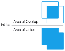
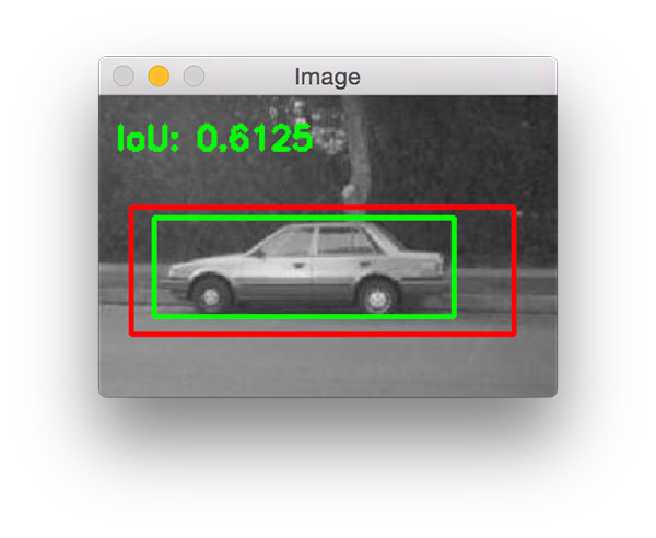
IOU metric (intersection over union metric)
- measure the performance of a model on the semantic segmentation task

11. Inference Performance

Bandwidth is the rate of data transfer, bit rate, or throughput, typically measured in bits per second.
Optimize:
- fusion
- quantization
- machine code compilation: Graph to binary
FPS:
- SS (Semantic system): 4-7 fps
- YOLO: 40-90 fps
Fusion
- Reduce the number of the oprations and accelarate the data passing through the graph
- eg: Batch Nomalization + Relu + Convolution --> BatchNorm/Relu/Conv
- save memory and time
Quantization
reduce precision from single precision --> half precision --> 8-bit network

12. Project: Semantic Segmantation Project

Paper: Fully Convolutional Networks for Semantic Segmentation
upsample
- Upsampling is interpolation, applied in the context of digital signal processing and sample rate conversion. When upsampling is performed on a sequence of samples of a continuous function or signal, it produces an approximation of the sequence that would have been obtained by sampling the signal at a higher rate (or density, as in the case of a photograph). For example, if compact disc audio is upsampled by a factor of 5/4, the resulting sample-rate increases from 44,100 Hz to 55,125 Hz.

23. Packages and Catkin Workspaces

rosdep
- The rosdep tool will check for a package's missing dependencies, download them, and install them.
  
  To check for missing dependencies in the simple_arm package:
```
$ rosdep check simple_arm
```
  Note: In order for the command to work, the workspace must be sourced.
  
  This gives you a list of the system dependencies that are missing, and where to get them.
  
  To have rosdep install packages, invoke the following command from the root of the catkin workspace
```
$ rosdep install -i simple_arm
```
  Issues with this command may arise when using a VM. If this is the case, please try:
```
$ sudo apt-get install ros-kinetic-gazebo-ros-control
```

24. Writting ROS Nodes

Common code entrance template:

if __name__ == '__main__':
    try:
        main_function()
    except rospy.ROSInterruptException:
        pass

Publisher

pub1 = rospy.Publisher("/topic_name", message_type, queue_size=size)

Subscriber

sub1 = rospy.Subscriber("/topic_name", message_type, callback_function)

Service ---- a request/respose mechanism

service = rospy.Service('service_name', serviceClassName, handler)

Using Service

service_proxy = rospy.ServiceProxy('service_name', serviceClassName)

Action Server & Client
How to choose Service and Action in different cases? (Think about it from avoiding congestion)

parameters

min_j1 = rospy.get_param('~min_joint_1_angle', 0)

Accordingly, in the launch file:

<node blablabla>
    <rosparam>
        min_joint_1_angle: 0
    </rosparam>
</node>

Logging
Additional Resources
- While we’ve done our best to give you a solid understanding of the fundamental concepts of ROS, the lessons here are by no means comprehensive. Fortunately, there are a wealth of resources available online.
- ROS Wiki
  - This is the official source of documentation for all ROS packages. Additionally, there are many helpful tutorials here. Aside from a simple search on google, this is probably the first place you should go if you are having a ROS-related problem.
- ROS Answers
  - If the wiki does not provide the answers you are looking for, ROS Answers will be the next best bet. With over 33,000 questions asked on ROS answers, there’s a good chance that somebody has already addressed the problem that you are dealing with.
- ROS Cheat Sheet
  - This is the official ROS cheat sheet. Even though the title indicates that it is for the indigo distribution, almost all of the commands still work in Kinetic, the distribution that we are using for this program.
- A gentle Introduction to ROS
  - This is a great book, and is distributed not only in paperback form, but also for free as a PDF download.

posted @ 2018-01-02 09:02 CasperWin 阅读(844) 评论(0) 编辑收藏举报

刷新页面返回顶部

卡斯柏的博客

笔下虽有千言，胸中实无一策