大作业

一、boston房价预测

1. 读取数据集

#导入包
from sklearn.model_selection import train_test_split
from sklearn.preprocessing import PolynomialFeatures
import pandas as pd
#导入数据集
from sklearn.datasets import load_boston
from sklearn.model_selection import train_test_split

2. 训练集与测试集划分 

#波士顿房价数据集
data = load_boston()
# 划分数据集
x_train, x_test, y_train, y_test = train_test_split(data.data,data.target,test_size=0.3)

3. 线性回归模型：建立13个变量与房价之间的预测模型，并检测模型好坏。

#建立模型
from sklearn.linear_model import LinearRegression
LR = LinearRegression()
LR.fit(x_train,y_train)
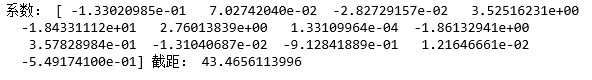
print('系数：',LR.coef_,"截距：",LR.intercept_)

　　运行结果：

 

#检测模型好坏
from sklearn.metrics import regression
y_predict = LR.predict(x_test)
# 计算模型的预测指标
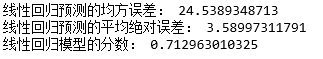
print("线性回归预测的均方误差：", regression.mean_squared_error(y_test,y_predict))
print("线性回归预测的平均绝对误差：", regression.mean_absolute_error(y_test,y_predict))
# 打印模型的分数
print("线性回归模型的分数：",LR.score(x_test, y_test))

　　运行结果：

 

4. 多项式回归模型：建立13个变量与房价之间的预测模型，并检测模型好坏。

# 多元多项式回归模型
# 多项式化
poly2 = PolynomialFeatures(degree=2)
x_poly_train = poly2.fit_transform(x_train)
x_poly_test = poly2.transform(x_test)
# 建立模型
LRP = LinearRegression()
LRP.fit(x_poly_train, y_train)

　　运行结果：

# 预测
y_predict2 = LRP.predict(x_poly_test)
# 检测模型好坏
# 计算模型的预测指标
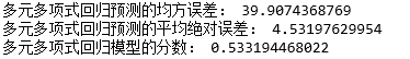
print("多元多项式回归预测的均方误差：", regression.mean_squared_error(y_test,y_predict2))
print("多元多项式回归预测的平均绝对误差：", regression.mean_absolute_error(y_test,y_predict2))
# 打印模型的分数
print("多元多项式回归模型的分数：",LRP.score(x_poly_test, y_test))

　　运行结果：

 

 5. 比较线性模型与非线性模型的性能，并说明原因。

线性模型可以是用曲线拟合样本，但是分类的决策边界一定是直线的。多项式模型是曲线形式，比线性回归模型更加贴近样本点分布的范围，误差值更小。

 

 

二、中文文本分类

#导入包
import os
import numpy as np
import sys
from datetime import datetime
import gc

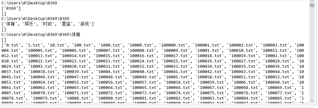
# 用os.walk获取需要的变量，并拼接文件路径再打开每一个文件
path = 'C:\\Users\\0\\Desktop\\0369'
for root,dirs,files in os.walk(path):
    print(root)
    print(dirs)
    print(files)
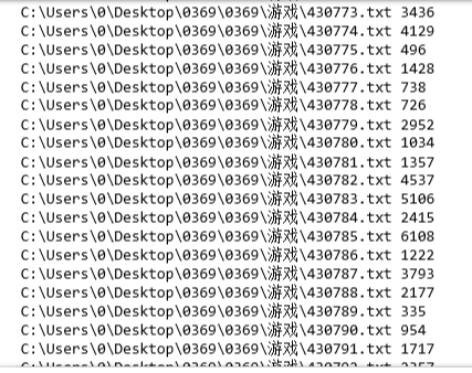
    for f in files:
        fn = os.path.join(root,f)
        size = os.path.getsize(fn)
        print(fn,size)

　　运行结果：

 

# 导入结巴库，并将需要用到的词库加进字典
import jieba
# 导入停用词：
with open(r'C:\Users\0\Desktop\stopsCN.txt', encoding='utf-8') as f:
    stopwords = f.read().split('\n')

def processing(tokens):
    # 去掉非字母汉字的字符
    tokens = "".join([char for char in tokens if char.isalpha()])
    # 结巴分词
    tokens = [token for token in jieba.cut(tokens,cut_all=True) if len(token) >=2]
    # 去掉停用词
    tokens = " ".join([token for token in tokens if token not in stopwords])
    return tokens

tokenList = []
targetList = []
# 用os.walk获取需要的变量，并拼接文件路径再打开每一个文件
for root,dirs,files in os.walk(path):
    for f in files:
        filePath = os.path.join(root,f)
        with open(filePath, encoding='utf-8') as f:
            content = f.read()
            # 获取新闻类别标签，并处理该新闻
        target = filePath.split('\\')[-2]
        targetList.append(target)
        tokenList.append(processing(content))

　

#将content_list列表向量化再建模，将模型用于预测并评估模型
# 划分训练集测试集并建立特征向量,为建立模型做准备
# 划分训练集测试集
from sklearn.feature_extraction.text import TfidfVectorizer
from sklearn.model_selection import train_test_split
from sklearn.naive_bayes import GaussianNB,MultinomialNB
from sklearn.model_selection import cross_val_score
from sklearn.metrics import classification_report
x_train,x_test,y_train,y_test = train_test_split(tokenList,targetList,test_size=0.2,stratify=targetList)
# 转化为特征向量，这里选择TfidfVectorizer的方式建立特征向量。不同新闻的词语使用会有较大不同。
vectorizer = TfidfVectorizer()
X_train = vectorizer.fit_transform(x_train)
X_test = vectorizer.transform(x_test)
# 建立模型,这里用多项式朴素贝叶斯，因为样本特征的a分布大部分是多元离散值
mnb = MultinomialNB()
module = mnb.fit(X_train, y_train)

#进行预测
y_predict = module.predict(X_test)
# 输出模型精确度
scores=cross_val_score(mnb,X_test,y_test,cv=5)
print("Accuracy:%.3f"%scores.mean())
# 输出模型评估报告
print("classification_report:\n",classification_report(y_predict,y_test))

　　运行结果：

 

#根据特征向量提取逆文本频率高的词汇,将预测结果和实际结果进行对比（用条形图）
# 将预测结果和实际结果进行对比
import collections
import matplotlib.pyplot as plt
from pylab import mpl
mpl.rcParams['font.sans-serif'] = ['FangSong'] # 指定默认字体  
mpl.rcParams['axes.unicode_minus'] = False # 解决保存图像是负号'-'显示为方块的问题

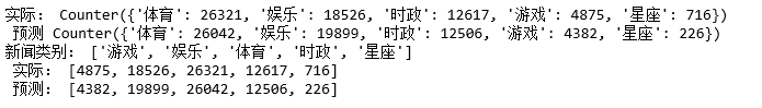
# 统计测试集和预测集的各类新闻个数
testCount = collections.Counter(y_test)
predCount = collections.Counter(y_predict)
print('实际：',testCount,'\n', '预测', predCount)

# 建立标签列表，实际结果列表，预测结果列表，
nameList = list(testCount.keys())
testList = list(testCount.values())
predictList = list(predCount.values())
x = list(range(len(nameList)))
print("新闻类别：",nameList,'\n',"实际：",testList,'\n',"预测：",predictList)

　　运行结果：

 

# 画图
plt.figure(figsize=(7,5))
total_width, n = 0.6, 2
width = total_width / n
plt.bar(x, testList, width=width,label='实际',fc = 'g')
for i in range(len(x)):
    x[i] = x[i] + width
plt.bar(x, predictList,width=width,label='预测',tick_label = nameList,fc='b')
plt.grid()
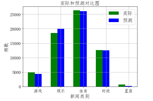
plt.title('实际和预测对比图',fontsize=17)
plt.xlabel('新闻类别',fontsize=17)
plt.ylabel('频数',fontsize=17)
plt.legend(fontsize =17)
plt.tick_params(labelsize=15)
plt.show()

　　运行结果：