激光数据匹配（MATLAB Robotics System Toolbox）

　　正态分布变换算法是一个配准算法，它应用于三维点的统计模型，使用标准最优化技术来确定两个点云间的最优的匹配，因为其在配准过程中不利用对应点的特征计算和匹配，所以时间比其他方法快。算法细节可以参考：NDT（Normal Distributions Transform）算法原理与公式推导。MATLAB  Robotics System Toolbox中的函数matchScans就是使用NDT算法来对两帧激光数据进行匹配，得到它们之间的相对变换关系。

 matchScans函数的用法 

　　matchScans函数用于匹配两帧激光雷达数据，输出两帧之间的姿态变换。用法主要有下面几种：

pose = matchScans(currScan,refScan) % finds the relative pose between a reference lidarScan and a current lidarScan object using the normal distributions transform (NDT).
pose = matchScans(currRanges,currAngles,refRanges,refAngles) % finds the relative pose between two laser scans specified as ranges and angles.
[pose,stats] = matchScans(___)                 % returns additional statistics about the scan match result using the previous input arguments.

 　　输出参数：

1. pose：Pose of current scan relative to the reference scan, returned as [x y theta], where [x y] is the translation in meters and theta is the rotation in radians.
2. stats：Scan matching statistics, returned as a structure with the following fields:

• • Score — Numeric scalar representing the NDT score while performing scan matching. This score is an estimate of the likelihood that the transformed current scan matches the reference scan. Score is always nonnegative. Larger scores indicate a better match.

• • Hessian — 3-by-3 matrix representing the Hessian of the NDT cost function at the given pose solution. The Hessian is used as an indicator of the uncertainty associated with the pose estimate.

 　　其它输入参数：

• 'SolverAlgorithm' ：Optimization algorithm, specified as either 'trust-region'(default) or 'fminunc'
• 'InitialPose'：Initial guess of the current pose relative to the reference laser scan, specified as the comma-separated pair consisting of 'InitialPose' and an [x y theta] vector. [0 0 0] (default)
• 'MaxIterations'：Maximum number of iterations, (400  default)
• 'ScoreTolerance'：Lower bound on the change in NDT score, specified as the comma-separated pair consisting of 'ScoreTolerance' and a numeric scalar. The NDT score is stored in the Score field of the output stats structure. Between iterations, if the score changes by less than this tolerance, the algorithm converges to a solution. A smaller tolerance results in more accurate pose estimates, but requires a longer execution time. (1e-6 default)
• 'CellSize'：Length of a cell side in meters (1 default). matchScans uses the cell size to discretize the space for the NDT algorithm. Tuning the cell size is important for proper use of the NDT algorithm. The optimal cell size depends on the input scans and the environment of your robot. Larger cell sizes can lead to less accurate matching with poorly sampled areas. Smaller cell sizes require more memory and less variation between subsequent scans. Sensor noise influences the algorithm with smaller cell sizes as well. Choosing a proper cell size depends on the scale of your environment and the input data.

 

•  Match Lidar Scans

　　首先使用lidarScan函数创建一个对象来存储2D激光扫描信息（Creat object for storing 2-D lidar scan），主要有下面3种使用方式：

% creates a lidarScan object from the ranges and angles, that represent the data collected from a lidar sensor. 
% The ranges and angles inputs are vectors of the same length and are set directly to the Ranges and Angles properties.
scan = lidarScan(ranges, angles)

scan = lidarScan(cart)     % creates a lidarScan object using the input Cartesian coordinates as an n-by-2 matrix. The Cartesian property is set directly from this input.
scan = lidarScan(scanMsg)  % creates a lidarScan object from a LaserScan ROS message object.

 　　我们按照距离—角度方式创建一个参考数据：

refRanges = 5*ones(1,300);
refAngles = linspace(-pi/2,pi/2,300);
refScan = lidarScan(refRanges,refAngles);

　　然后使用transformScan将参考激光数据变换到另一个位置：

currScan = transformScan(refScan,[0.5 0.2 0]);  % transforms the laser scan by using the specified relative pose

　　下面使用matchScans函数来计算这两帧数据之间的相对变换：

pose = matchScans(currScan,refScan);

　　结果为：pose = -0.4999   -0.2092   0.0185 

　　最后可以再使用transformScan根据计算出的pose对第二帧数据进行变换，看看与第一帧数据的重合程度怎么样：

currScan2 = transformScan(currScan,pose);

subplot(2,1,1);
hold on
plot(currScan)
plot(refScan)
title('Original Scans')
hold off

subplot(2,1,2);
hold on
plot(currScan2)
plot(refScan)
title('Aligned Scans')
xlim([0 5])
hold off

 　　从下图可以看出两帧数据匹配的很好：

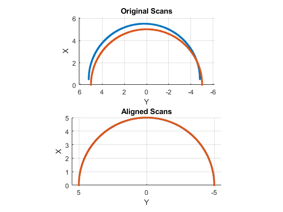
• Match Laser Scans

 　　Specify a reference laser scan as ranges and angles：

refRanges = 5*ones(1,300);
refAngles = linspace(-pi/2,pi/2,300);

　　使用transformScan函数对参考数据进行变换，生成第二个激光数据：

[currRanges,currAngles] = transformScan(refRanges,refAngles,[0.5 0.2 0]);

 　　调用matchScans函数时还可以指定其它参数，比如求解方法，初值，迭代次数等（Specify optional comma-separated pairs of Name,Value arguments. Name is the argument name and Value is the corresponding value. Name must appear inside single quotes (' '). You can specify several name and value pair arguments in any order asName1,Value1,...,NameN,ValueN.）

pose = matchScans(currRanges,currAngles,refRanges,refAngles,'SolverAlgorithm','fminunc');

　　pose = -0.5417  0.0165  -0.4096，可以看出误差比较大

　　通过指定初始值可以提高准确度（Improve the estimate by giving an initial pose estimate.）

pose = matchScans(currRanges,currAngles,refRanges,refAngles,'SolverAlgorithm','fminunc','InitialPose',[-0.4 -0.1 0]);

　　pose = -0.5100  -0.1834  -0.0330，比没有指定初值的结果要好很多

　　最后再根据计算出的结果将第2帧数据变换回去，进行对比：

[currRanges2,currAngles2] = transformScan(currRanges,currAngles,pose);

[x1 y1] = pol2cart(refAngles,refRanges);
[x2 y2] = pol2cart(currAngles,currRanges);
[x3 y3] = pol2cart(currAngles2,currRanges2);

subplot(1,2,1)
plot(x1,y1,'o',x2,y2,'*r')
title('Original Scans')
subplot(1,2,2)
plot(x1,y1,'o',x3,y3,'*r')
title('Aligned Scans')

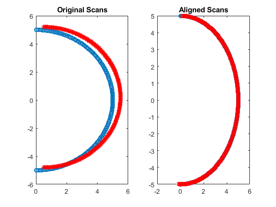
 Estimate Robot Pose with Scan Matching 

　　The goal of scan matching is to find the relative pose (or transform) between the two robot positions where the scans were taken. The scans can be aligned based on the shapes of their overlapping features. To estimate this pose, NDT subdivides the laser scan into 2D cells and each cell is assigned a corresponding normal distribution. The distribution represents the probability of measuring a point in that cell. Once the probability density is calculated, an optimization method finds the relative pose between the current laser scan and the reference laser scan. To speed up the convergence of the method, an initial guess of the pose can be provided. Typically, robot odometry is used to supply the initial estimate.

　　If you apply scan matching to a sequence of scans, you can use it to recover a rough map of the environment that the robot traverses. Scan matching also plays a crucial role in other applications, such as position tracking and Simultaneous Localization and Mapping (SLAM).

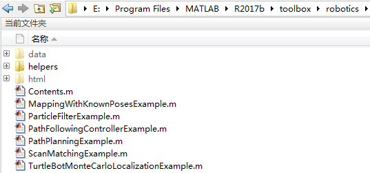
　　我们可以通过匹配激光扫描数据来估计机器人位姿。下面看一个例子，将工作目录切换到Program Files\MATLAB\R2017b\toolbox\robotics\robotexamples\robotalgs下：

　　加载激光扫描数据文件：

filePath = fullfile(fileparts(mfilename('fullpath')), 'data', 'scanMatchingData.mat');
load(filePath);

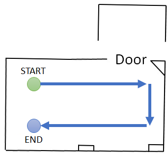
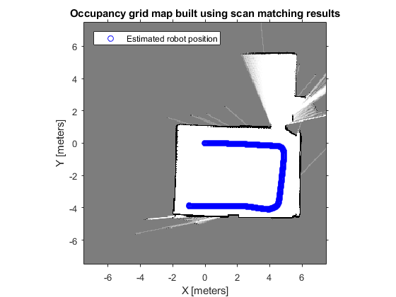
 　　激光数据由室内移动机器人采集，机器人的大致移动路径如下图所示：

　　下面我们从laserMsg中挑选相隔比较近的两帧数据，画出来看看：

referenceScan = lidarScan(laserMsg{180});
currentScan = lidarScan(laserMsg{202});

currScanCart = currentScan.Cartesian;
refScanCart = referenceScan.Cartesian;
figure
plot(refScanCart(:,1), refScanCart(:,2), 'k.');
hold on
plot(currScanCart(:,1), currScanCart(:,2), 'r.');
legend('Reference laser scan', 'Current laser scan', 'Location', 'NorthWest');

　　由于这两帧数据间隔比较近，所以它们之间会存在许多相同的特征。They should share common features by being close together in the sequence.

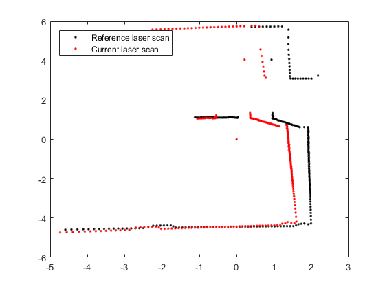
　　使用matchScans计算这两帧数据间的变换关系：

transform = matchScans(currentScan, referenceScan)

transform =

    0.5348   -0.0065   -0.0336

 　　为了验证相对变换的计算是否正确，可以用transformScan函数将currentScan变换回去查看两帧数据是否重合。This transformed laser scan can be used to visualize the result.

transScan = transformScan(currentScan, transform);

　　下面画出两帧激光数据图像：

figure
plot(refScanCart(:,1), refScanCart(:,2), 'k.');
hold on
transScanCart = transScan.Cartesian;
plot(transScanCart(:,1), transScanCart(:,2), 'r.');
legend('Reference laser scan', 'Transformed current laser scan', 'Location', 'NorthWest');

　　如果计算出的变换比较准确，那两帧图像会匹配的很好。If the scan matching was successful, the two scans should be well-aligned.

 Build Occupancy Grid Map Using Iterative Scan Matching

 　　如果我们对一些列连续的激光数据进行匹配，那么我们就能够从这些信息中粗略的建立环境地图（If you apply scan matching to a sequence of scans, you can use it to recover a rough map of the environment）。下面看一个例子，新建一个15m×15m的空地图，设置地图原点在[-7.5 -7.5]处：

map = robotics.OccupancyGrid(15, 15, 20);
map.GridLocationInWorld = [-7.5 -7.5]

map = 

  OccupancyGrid with properties:

        OccupiedThreshold: 0.6500
            FreeThreshold: 0.2000
    ProbabilitySaturation: [0.0010 0.9990]
                 GridSize: [300 300]
               Resolution: 20
             XWorldLimits: [-7.5000 7.5000]
             YWorldLimits: [-7.5000 7.5000]
      GridLocationInWorld: [-7.5000 -7.5000]

 　　每一帧激光扫描数据都对应着一个机器人的位姿，我们要通过激光数据之间的匹配关系来推算机器人的运动。以第一帧数据为参考位置，假设机器人位姿的初始值为[0 0 0]。预先分配一个矩阵poseList用于存储机器人运动路径上的位置和姿态：

numScans = numel(laserMsg);
initialPose = [0 0 0];  % Typically, robot odometry is used to supply the initial estimate.
poseList = zeros(numScans,3);
poseList(1,:) = initialPose;
transform = initialPose;

 　　下面的代码循环处理所有激光数据，计算出相邻两帧之间的变换后通过exampleHelperComposeTransform函数计算出机器人相对于初始参考点的绝对位姿，并使用robotics.OccupancyGrid.insertRay函数来更新地图：

% Loop through all the scans and calculate the relative poses between them
for idx = 2:numScans
    % Process the data in pairs.
    referenceScan = lidarScan(laserMsg{idx-1});
    currentScanMsg = laserMsg{idx};
    currentScan = lidarScan(currentScanMsg);

    % Run scan matching. Note that the scan angles stay the same and do
    % not have to be recomputed. To increase accuracy, set the maximum
    % number of iterations to 500. Use the transform from the last
    % iteration as the initial estimate.
    [transform, stats] = matchScans(currentScan, referenceScan, ...
        'MaxIterations', 500, 'InitialPose', transform);

    % The |Score| in the statistics structure is a good indication of the quality of the scan match.
    if stats.Score / currentScan.Count < 1.0
        disp(['Low scan match score for index ' num2str(idx) '. Score = ' num2str(stats.Score) '.']);
    end

    % Maintain the list of robot poses.
    absolutePose = exampleHelperComposeTransform(poseList(idx-1,:), transform);
    poseList(idx,:) = absolutePose;

    % Integrate the current laser scan into the probabilistic occupancy grid.
    insertRay(map, absolutePose, currentScan, double(currentScanMsg.RangeMax));
end

　　exampleHelperComposeTransform函数内容如下：

function composedTransform = exampleHelperComposeTransform(baseTransform, relativeTransform)
　　%exampleHelperComposeTransform Compose two transforms
　　%   The RELATIVETRANSFORM is added to the BASETRANSFORM and the composed
　　%   transform is returned in COMPOSEDTRANSFORM.
　　%   BASETRANSFORM is the transform from laser scan 1 to world and
　　%   RELATIVETRANSFORM is the transform from laser scan 2 to laser scan
　　%   1 (as returned by matchScans).

　　% Concatenate the 4x4 homogeneous transform matrices for the base and
　　% relative transforms.
　　tform = pose2tform(baseTransform) * pose2tform(relativeTransform);

　　% Extract the translational vector
　　trvec = tform2trvec(tform);

　　% Extract the yaw angle from the resulting transform
　　eul = tform2eul(tform);
　　theta = eul(1);  % The default order for Euler angle rotations is 'ZYX'

　　% Composed transform has structure [x y theta(z-axis)]
　　composedTransform = [trvec(1:2) theta];
end


function tform = pose2tform(pose)
　　%pose2tform Convert [x y theta] pose into homogeneous transform
　　%   TFORM is returned as a 4x4 matrix.

　　x = pose(1);
　　y = pose(2);
　　theta = pose(3);
　　tform = trvec2tform([x y 0]) * eul2tform([theta 0 0]);
end

　　显示建好的地图：

figure
show(map);
title('Occupancy grid map built using scan matching results');

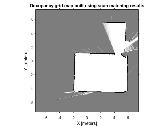
　　最后可以绘制出机器人在地图中的运动路径。 Plot the absolute robot poses that were calculated by the scan matching algorithm. This shows the path that the robot took through the map of the environment.

hold on
plot(poseList(:,1), poseList(:,2), 'bo', 'DisplayName', 'Estimated robot position');

 

参考：

matchScans

Scan matching

NDT方法在SLAM中的应用

Estimate Robot Pose with Scan Matching

Compose a Series of Laser Scans with Pose Changes

NDT（Normal Distributions Transform）算法原理与公式推导

使用正态分布变换（Normal Distributions Transform）进行点云配准

The Normal Distributions Transform: A New Approach to Laser Scan Matching